22.1.4.3 Mathematical Considerations

The attempt has been made to make sparse matrices behave in exactly the same manner as there full counterparts. However, there are certain differences and especially differences with other products sparse implementations.

Firstly, the "./" and ".^" operators must be used with care. Consider what the examples

       s = speye (4);
       a1 = s .^ 2;
       a2 = s .^ s;
       a3 = s .^ -2;
       a4 = s ./ 2;
       a5 = 2 ./ s;
       a6 = s ./ s;

will give. The first example of s raised to the power of 2 causes no problems. However s raised element-wise to itself involves a a large number of terms 0 .^ 0 which is 1. There s .^ s is a full matrix.

Likewise s .^ -2 involves terms terms like 0 .^ -2 which is infinity, and so s .^ -2 is equally a full matrix.

For the "./" operator s ./ 2 has no problems, but 2 ./ s involves a large number of infinity terms as well and is equally a full matrix. The case of s ./ s involves terms like 0 ./ 0 which is a NaN and so this is equally a full matrix with the zero elements of s filled with NaN values.

The above behavior is consistent with full matrices, but is not consistent with sparse implementations in other products.

A particular problem of sparse matrices comes about due to the fact that as the zeros are not stored, the sign-bit of these zeros is equally not stored. In certain cases the sign-bit of zero is important. For example

      a = 0 ./ [-1, 1; 1, -1];
      b = 1 ./ a
      => -Inf            Inf
          Inf           -Inf
      c = 1 ./ sparse (a)
      =>  Inf            Inf
          Inf            Inf

To correct this behavior would mean that zero elements with a negative sign-bit would need to be stored in the matrix to ensure that their sign-bit was respected. This is not done at this time, for reasons of efficient, and so the user is warned that calculations where the sign-bit of zero is important must not be done using sparse matrices.

In general any function or operator used on a sparse matrix will result in a sparse matrix with the same or a larger number of non-zero elements than the original matrix. This is particularly true for the important case of sparse matrix factorizations. The usual way to address this is to reorder the matrix, such that its factorization is sparser than the factorization of the original matrix. That is the factorization of L * U = P * S * Q has sparser terms L and U than the equivalent factorization L * U = S.

Several functions are available to reorder depending on the type of the matrix to be factorized. If the matrix is symmetric positive-definite, then symamd or csymamd should be used. Otherwise colamd or ccolamd should be used. For completeness the reordering functions colperm and randperm are also available.

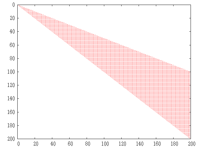
See fig:simplematrix, for an example of the structure of a simple positive definite matrix.

Figure 22.3: Structure of simple sparse matrix.

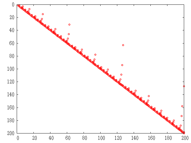
The standard Cholesky factorization of this matrix, can be obtained by the same command that would be used for a full matrix. This can be visualized with the command r = chol(A); spy(r);. See fig:simplechol. The original matrix had 598 non-zero terms, while this Cholesky factorization has 10200, with only half of the symmetric matrix being stored. This is a significant level of fill in, and although not an issue for such a small test case, can represents a large overhead in working with other sparse matrices.

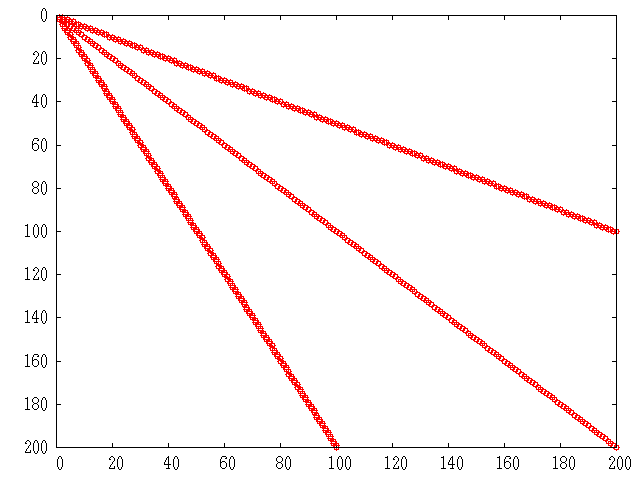
The appropriate sparsity preserving permutation of the original matrix is given by symamd and the factorization using this reordering can be visualized using the command q = symamd(A); r = chol(A(q,q)); spy(r). This gives 399 non-zero terms which is a significant improvement.

The Cholesky factorization itself can be used to determine the appropriate sparsity preserving reordering of the matrix during the factorization, In that case this might be obtained with three return arguments as r[r, p, q] = chol(A); spy(r).

Figure 22.4: Structure of the un-permuted Cholesky factorization of the above matrix.

Figure 22.5: Structure of the permuted Cholesky factorization of the above matrix.

In the case of an asymmetric matrix, the appropriate sparsity preserving permutation is colamd and the factorization using this reordering can be visualized using the command q = colamd(A); [l, u, p] = lu(A(:,q)); spy(l+u).

Finally, Octave implicitly reorders the matrix when using the div (/) and ldiv (\) operators, and so no the user does not need to explicitly reorder the matrix to maximize performance.