22.1.3 Finding out Information about Sparse Matrices

There are a number of functions that allow information concerning sparse matrices to be obtained. The most basic of these is issparse that identifies whether a particular Octave object is in fact a sparse matrix.

Another very basic function is nnz that returns the number of non-zero entries there are in a sparse matrix, while the function nzmax returns the amount of storage allocated to the sparse matrix. Note that Octave tends to crop unused memory at the first opportunity for sparse objects. There are some cases of user created sparse objects where the value returned by nzmaz will not be the same as nnz, but in general they will give the same result. The function spstats returns some basic statistics on the columns of a sparse matrix including the number of elements, the mean and the variance of each column.

When solving linear equations involving sparse matrices Octave determines the means to solve the equation based on the type of the matrix as discussed in Sparse Linear Algebra. Octave probes the matrix type when the div (/) or ldiv (\) operator is first used with the matrix and then caches the type. However the matrix_type function can be used to determine the type of the sparse matrix prior to use of the div or ldiv operators. For example

     a = tril (sprandn(1024, 1024, 0.02), -1) ...
         + speye(1024);
     matrix_type (a);
     ans = Lower

show that Octave correctly determines the matrix type for lower triangular matrices. matrix_type can also be used to force the type of a matrix to be a particular type. For example

     a = matrix_type (tril (sprandn (1024, ...
        1024, 0.02), -1) + speye(1024), 'Lower');

This allows the cost of determining the matrix type to be avoided. However, incorrectly defining the matrix type will result in incorrect results from solutions of linear equations, and so it is entirely the responsibility of the user to correctly identify the matrix type

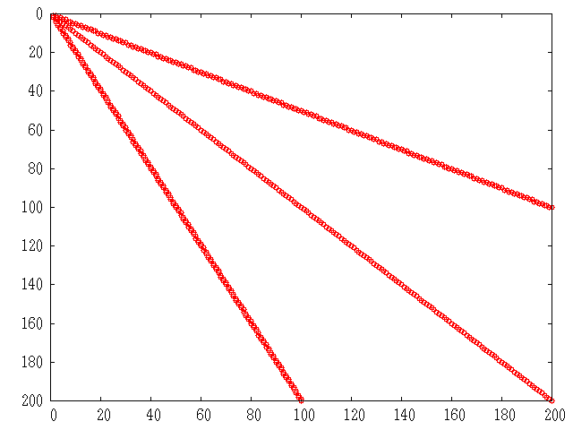
There are several graphical means of finding out information about sparse matrices. The first is the spy command, which displays the structure of the non-zero elements of the matrix. See fig:spmatrix, for an exaple of the use of spy. More advanced graphical information can be obtained with the treeplot, etreeplot and gplot commands.

Figure 22.1: Structure of simple sparse matrix.

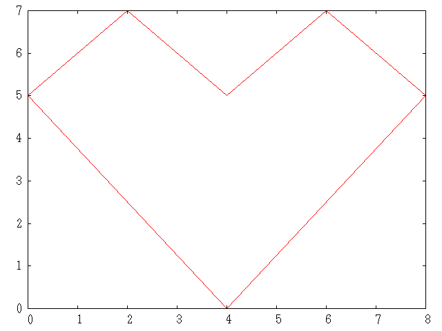
One use of sparse matrices is in graph theory, where the interconnections between nodes is represented as an adjacency matrix. That is, if the i-th node in a graph is connected to the j-th node. Then the ij-th node (and in the case of undirected graphs the ji-th node) of the sparse adjacency matrix is non-zero. If each node is then associated with a set of co-ordinates, then the gplot command can be used to graphically display the interconnections between nodes.

As a trivial example of the use of gplot, consider the example

     A = sparse([2,6,1,3,2,4,3,5,4,6,1,5],
         [1,1,2,2,3,3,4,4,5,5,6,6],1,6,6);
     xy = [0,4,8,6,4,2;5,0,5,7,5,7]';
     gplot(A,xy)

which creates an adjacency matrix A where node 1 is connected to nodes 2 and 6, node 2 with nodes 1 and 3, etc. The co-ordinates of the nodes are given in the n-by-2 matrix xy. See fig:gplot.

Figure 22.2: Simple use of the gplot command.

The dependencies between the nodes of a Cholesky factorization can be calculated in linear time without explicitly needing to calculate the Cholesky factorization by the etree command. This command returns the elimination tree of the matrix and can be displayed graphically by the command treeplot(etree(A)) if A is symmetric or treeplot(etree(A+A')) otherwise.